PReFlow: Learning to Refine Diffusion Policies

Proposal-conditioned flows for expressive, efficient policy improvement in offline and offline-to-online reinforcement learning.

Overview

A behavior policy offers a useful starting action. But selecting the best action it samples can still leave room for improvement: better actions may lie nearby, and there may be several different ways to improve the same proposal.

Proposal-Conditioned Refinement Flows (PReFlow) learns a distribution of these improvements. A behavior flow proposes actions, a critic selects a promising proposal, and a second, conditional flow refines it. This post explains our paper, Diffusion Policy Improvement with Proposal-Conditioned Refinement Flows, by Junhyun Ha, Juho Lee, and Byoungwoo Park.

Paper on arXiv PDF BibTeX

Figure 1 from the paper. Left: different ways of improving a behavior policy. Right: aggregate success rates after offline training and online fine-tuning. PReFlow reaches a mean of 91% after 500K online environment steps.

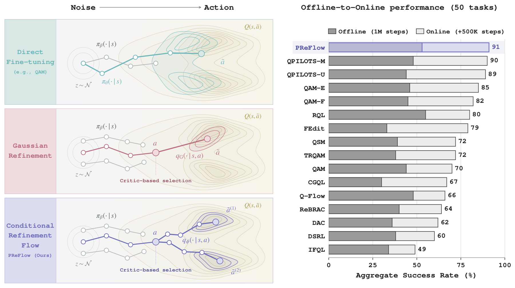
The method has two useful properties: the refinement can represent multiple separated modes, and its training targets have a closed form. The latter removes the need for a backward adjoint solve when training the refinement flow.

Why refine a proposal

In offline reinforcement learning, a critic \(Q_\psi(s,a)\) estimates which actions are valuable, while a behavior policy \(\pi_\beta(a\mid s)\) models the actions supported by the dataset. A common policy improvement objective balances value against a KL penalty toward that behavior policy:

\[\max_\pi\; \mathbb{E}_{\tilde a\sim\pi(\cdot\mid s)} \left[Q_\psi(s,\tilde a)\right] -\frac{1}{\tau}\operatorname{KL}(\pi\Vert\pi_\beta).\]

At a fixed state, its optimum is

\[\pi^\star(\tilde a\mid s) \propto \pi_\beta(\tilde a\mid s) \exp\!\left(\tau Q_\psi(s,\tilde a)\right).\]

The behavior-density factor matters: even a high-value action receives little weight if its behavior density is small. This can discourage useful changes near a likely behavior action.

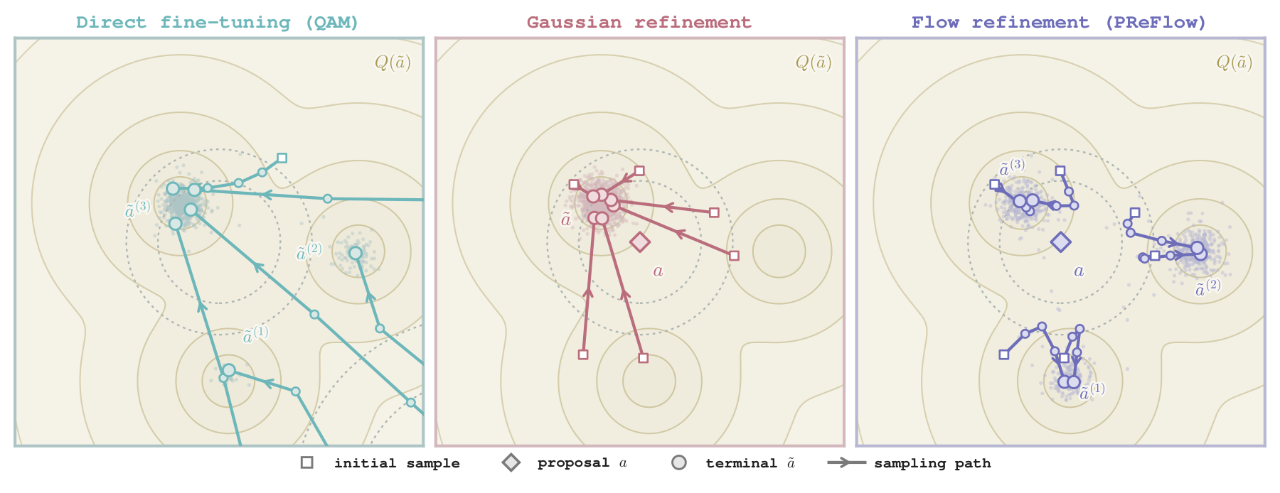
An alternative is to sample an action first, then improve it locally. But the choice of refinement distribution matters too. A deterministic editor produces one refinement; a Gaussian editor cannot represent several separated modes for a fixed state and proposal. A conditional flow gives the refinement distribution more flexibility.

Figure 2 from the paper. In this toy experiment, PReFlow represents three high-value modes around a proposal. The Gaussian editor concentrates on one, while direct fine-tuning undercovers the two modes farther from the proposal.

Select then refine

At a state \(s\), action generation has three steps:

1. Sample \(K\) candidate actions from the behavior flow.
2. Select the candidate with the highest critic value.
3. Sample a refinement from a flow conditioned on both the state and the selected proposal.

Writing the selected proposal as \(a\) and the refinement as \(\Delta a\), the executed action is

\[\tilde a = a+\Delta a.\]

We regularize the refined-action distribution toward \(\mathcal N(a,\delta^2 I)\). The scale \(\delta\) controls the reference neighborhood around the proposal. For a fixed proposal, the optimal refinement distribution is

\[\pi^{\mathrm{ref},\star}(\Delta a\mid s,a) \propto \exp\!\left( \tau Q_\psi(s,a+\Delta a) -\frac{\|\Delta a\|^2}{2\delta^2} \right).\]

The first term favors value; the second discourages large changes. Although the reference is Gaussian, the optimal refinement need not be: several peaks in the critic can produce several useful refinement modes.

A smoother behavior prior

The two stages also have a joint interpretation. Define the value of a proposal after optimal regularized refinement as

\[V_\delta(s,a) =\frac{1}{\tau}\log \mathbb{E}_{\Delta a\sim\mathcal N(0,\delta^2I)} \left[\exp\!\left(\tau Q_\psi(s,a+\Delta a)\right)\right].\]

If both proposal selection and refinement are optimized with the same KL coefficient, the final action distribution is

\[\pi_\delta^\star(\tilde a\mid s) \propto \bar\pi_{\beta,\delta}(\tilde a\mid s) \exp\!\left(\tau Q_\psi(s,\tilde a)\right),\]

where

\[\bar\pi_{\beta,\delta}(\tilde a\mid s) =\int \pi_\beta(a\mid s)\, \mathcal N(\tilde a;a,\delta^2I)\,\mathrm da.\]

This is policy improvement under a Gaussian-smoothed behavior prior. Nearby behavior proposals can supply reference density to an action even when its original behavior density is low.

This result describes the ideal joint optimum. The practical algorithm approximates proposal quality using \(Q_\psi(s,a)\) with taylor expansion, and chooses greedily among finitely many samples.

Training the refinement flow

We parameterize the refinement flow as \(\Delta a=\delta y_1\), where \(y_1\) is the endpoint of this conditional flow:

\[\frac{\mathrm dY_t}{\mathrm dt} =v_\varphi(Y_t,t\mid s,a), \qquad Y_0\sim\mathcal N(0,I).\]

The Gaussian refinement reference makes the training target especially simple. Given a sampled endpoint \(y_1\), draw \(t\sim\mathcal U(0,1)\) and fresh Gaussian noise \(\epsilon\), then construct

\[y_t=ty_1+(1-t)\epsilon, \qquad d(t)=t^2+(1-t)^2.\]

The adjoint-matching velocity target is

\[v^{\mathrm{tgt}} =\frac{2t-1}{d(t)}y_t +\frac{\tau\delta(1-t)}{d(t)} \nabla_{\tilde a}Q_\psi(s,a+\delta y_1).\]

Training the refiner then uses a single velocity regression loss:

\[\mathcal L_{\mathrm{actor}}(\varphi) =\mathbb E\left[ \left\|v_\varphi(y_t,t\mid s,a) -\operatorname{sg}[v^{\mathrm{tgt}}]\right\|_2^2 \right].\]

Here \(\operatorname{sg}\) denotes stop-gradient. For refinement training, proposals are sampled directly from the behavior policy with \(K=1\).

Our simulation-free construction only needs one forward flow rollout to generate an endpoint, and optimize efficiently via an endpoint critic gradient, no requirement of backward integration of adjoint dynamics. At inference, the critic scores proposals; the learned refinement flow does not require critic-gradient evaluations.

Results on OGBench

We evaluate on 50 tasks across ten OGBench domain variants. The main protocol uses 1M offline gradient steps, followed by 500K online environment steps. PReFlow and the reproduced baselines use eight seeds per task.

The table below reproduces a subset of the aggregate results in Table 1 of the paper. Entries are mean success rates, with reported 95% confidence intervals in brackets.

Method	Offline	After online fine-tuning
QAM-E	46% [45, 47]	85% [84, 86]
QPILOTS-U	44% [42, 47]	89% [87, 90]
QPILOTS-M	48% [46, 50]	90% [87, 91]
Q-Flow	48% [47, 48]	66% [65, 67]
RQL	55% [53, 56]	80% [80, 81]
PReFlow	53% [51, 54]	91% [90, 92]

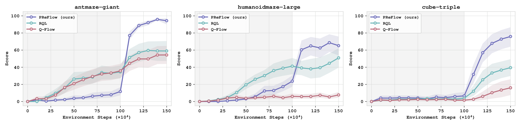
PReFlow has the highest aggregate online mean among the methods compared in the paper. RQL starts with a higher aggregate offline mean, but the ranking changes after online fine-tuning. Figure 3 examines this adaptation on antmaze-giant, humanoidmaze-large, and cube-triple. The full paper reports all baselines and individual domains.

Figure 3 from the paper. These illustrative curves use three seeds, with pointwise 95% confidence intervals. Online fine-tuning begins after 1M offline gradient steps; the plot uses a combined training axis.

Why might PReFlow adapt better online?

Section 5.1 offers a mechanistic hypothesis: an updated critic can affect both refinement learning and proposal selection directly. Q-Flow fits a value function at intermediate flow states using endpoint critic values, then uses its gradients to train the policy. RQL learns values for individual flow steps in an expanded MDP, using reversed flow trajectories for off-policy learning. Both methods therefore learn value information within the flow trajectory.

PReFlow constructs its refinement target from the critic gradient at the final action, \(\nabla_{\tilde a}Q_\psi(s,\tilde a)\). When online data improves the critic, that new signal can enter the next refinement regression target directly, without fitting an auxiliary intermediate-state value function. The same updated critic also changes which behavior proposal wins the selection step. These two routes provide a plausible explanation for the online gains in Figure 3, even when the offline starting score is modest.

Refinement ablation

To isolate refinement from candidate selection, Table 2 fixes one proposal, \(K=1\). The base policy executes that proposal directly. The other variants use a learned diagonal Gaussian or a conditional flow to refine it, with the same conditional objective and refinement scale \(\delta=0.1\).

The table reproduces offline success rates (%) after 1M gradient steps, including the paper’s reported \(\pm\) values. Each domain covers five tasks, with three seeds per task.

Domain	Base	Gaussian	Flow
antmaze-large	2.3 ± 0.8	76.3 ± 7.2	79.0 ± 7.5
humanoidmaze-medium	2.7 ± 1.0	57.1 ± 8.5	69.2 ± 1.2
scene	3.9 ± 1.5	68.1 ± 3.2	73.1 ± 0.8
cube-double	2.0 ± 0.0	40.8 ± 5.2	53.9 ± 3.3

Both refiners substantially improve the behavior proposal. Flow refinement has the higher mean in all four domains. Because \(K=1\) throughout, these gains support the benefit of the refinement policy class independently of choosing among more proposals.

Figure 8 from the paper. Refinement enabled (left, δ = 0.1) versus disabled (right, δ = 0), averaged over antmaze-large, humanoidmaze-medium, scene, and cube-double. This is an offline-only experiment through 1M gradient steps. Curves average three seeds; shading shows pointwise 95% confidence intervals.

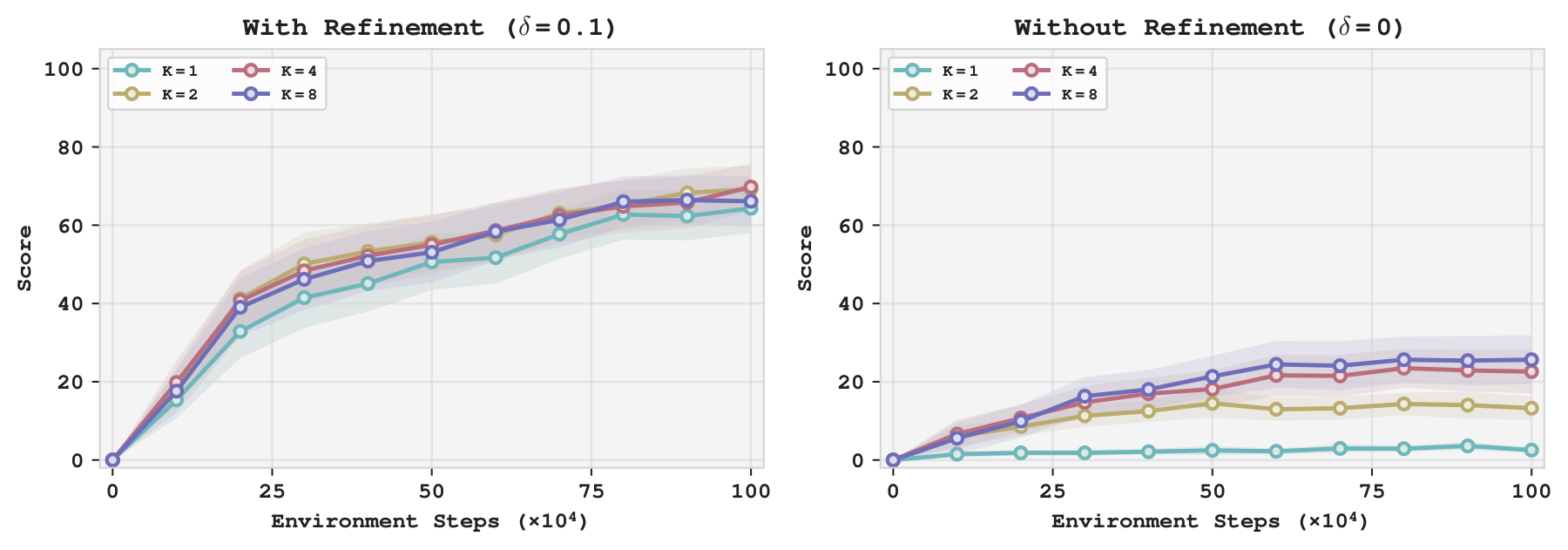
Figure 8 asks a complementary question: can more selection compensate for removing refinement? Selecting among more behavior proposals helps, but even \(K=8\) without refinement remains well below refinement with \(K=1\). In this controlled comparison, refinement accounts for most of the improvement, with selection providing an additional gain.

Selection ablation

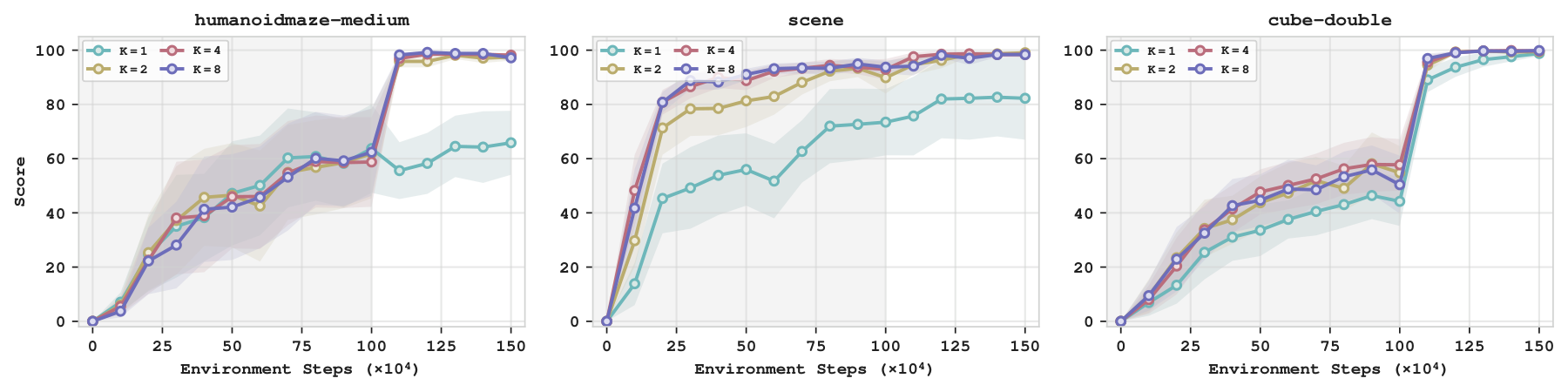
We next keep the learned refiner and vary the number of behavior proposals, \(K\in\{1,2,4,8\}\). With \(K=1\), the single proposal is refined directly. For \(K>1\), the critic selects the highest-value proposal before refinement. Figure 5 shows that selection can improve both offline learning and final online performance, with benefits already visible at \(K=2\).

Figure 5 from the paper. Proposal-count ablation with refinement in every setting. Online fine-tuning starts after 1M offline gradient steps; the horizontal axis combines offline and online training. Curves average three seeds; shading shows pointwise 95% confidence intervals. Full ten-domain curves appear in Appendix E.3.

Training cost

Figure 4 from the paper. Full training update times on one NVIDIA RTX A6000, averaged over 5, 10, 20, 50, and 100 flow steps. This measures training updates, not deployment latency.

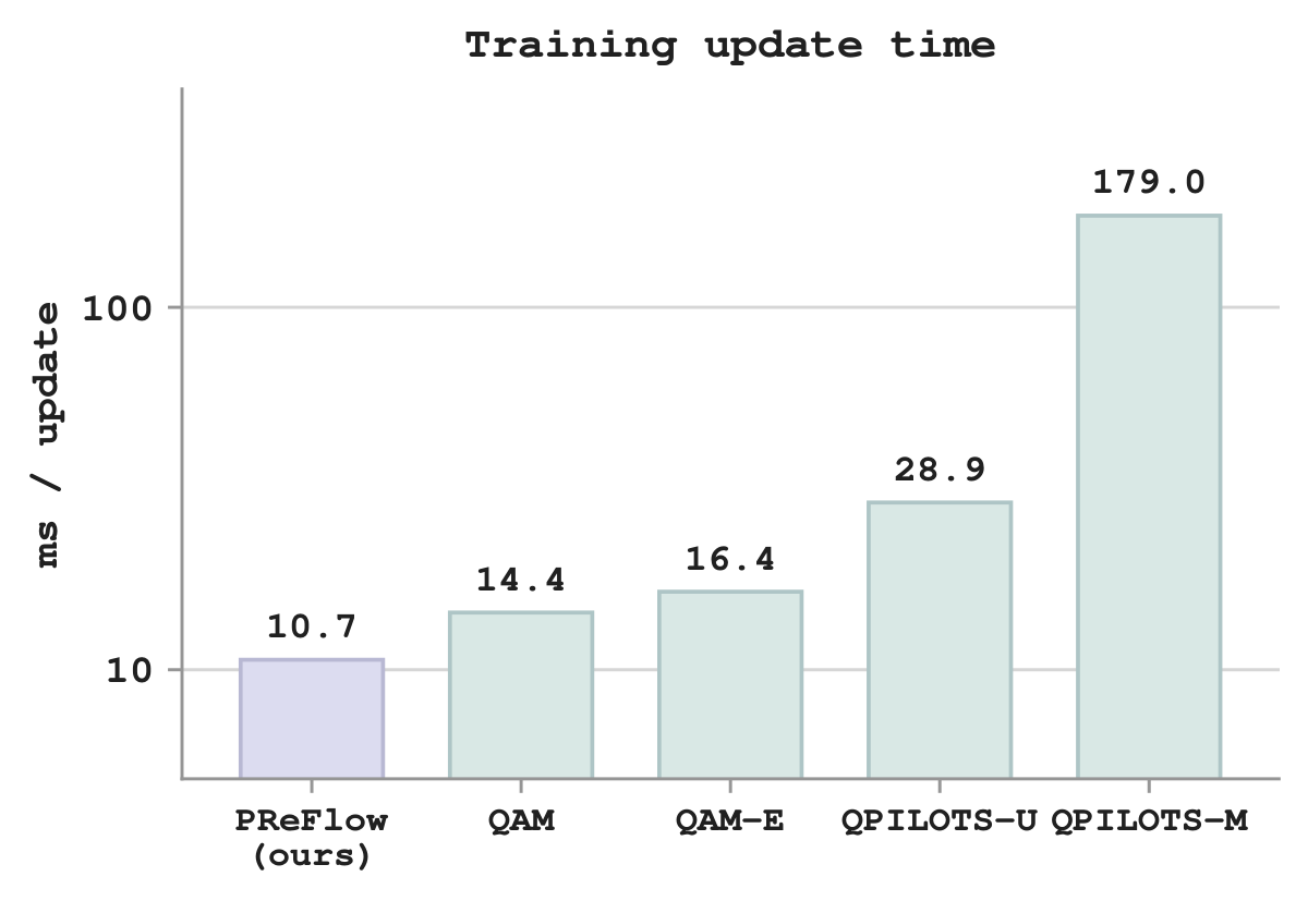
Under this timing protocol, PReFlow has the lowest mean full-update time among the compared methods. The closed-form target avoids the sequential backward adjoint computation used by QAM.

Paper and citation

Diffusion Policy Improvement with Proposal-Conditioned Refinement Flows
Junhyun Ha, Juho Lee, and Byoungwoo Park · arXiv preprint, September 2026

Read the paper for proofs, the complete training algorithm, hyperparameters, and per-task results.

@misc{ha2026preflow,
  title         = {Diffusion Policy Improvement with
                   Proposal-Conditioned Refinement Flows},
  author        = {Junhyun Ha and Juho Lee and Byoungwoo Park},
  year          = {2026},
  eprint        = {2609.36812},
  archivePrefix = {arXiv},
  primaryClass  = {cs.LG},
  url           = {https://arxiv.org/abs/2609.36812}
}